Billie Eilish reveals that the title of her new album comes from a Logic Pro synth name that doesn’t exist
Do you know which synth or preset she could have been thinking of?
Do you know which synth or preset she could have been thinking of?

“A lot of people ask why I don’t use the Neve on her," says Stuart White. "And I love the Neve on vocals, don’t get me wrong, but the Neves tend to crackle when you turn the pre gain”
An Oberheim and Minimoog went for a song, but it was a Martin Gore guitar and E-mu sampler that stole the show

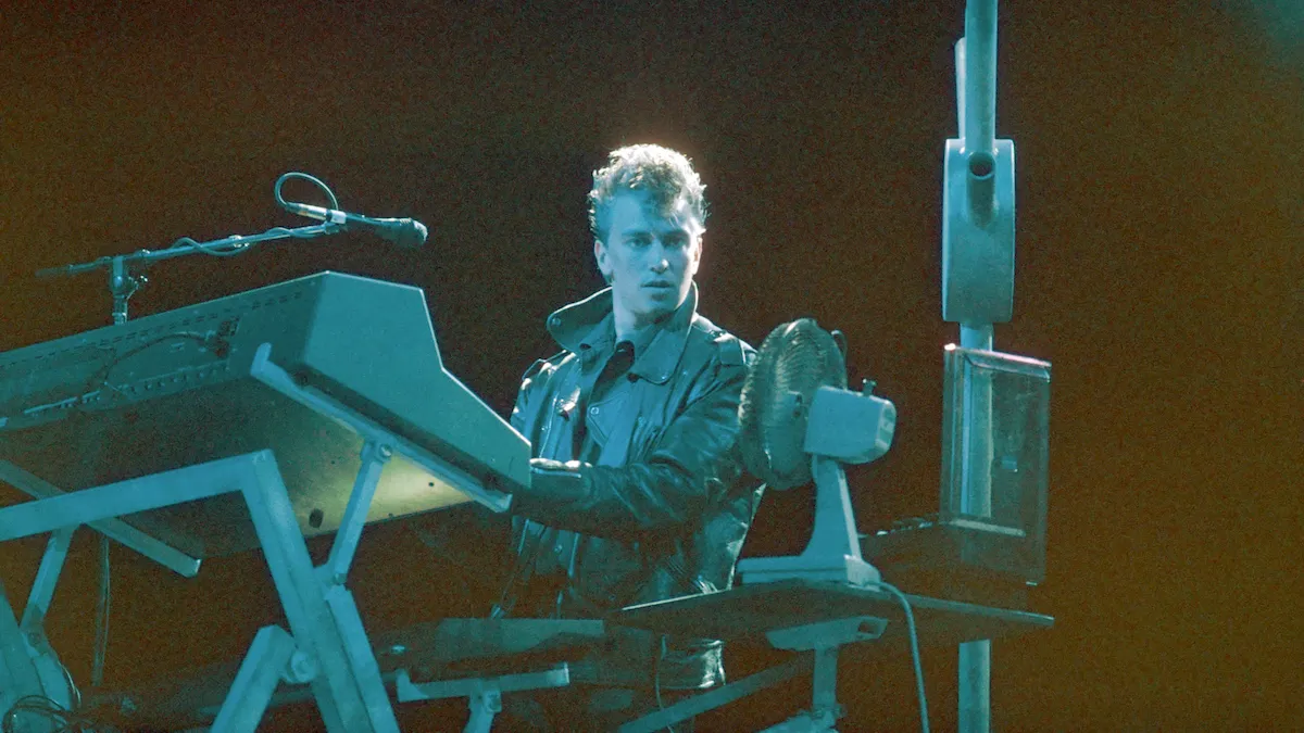
Near-death experiences, breakdowns, talking puppets, heart attacks, sleeping in coffins… Just another Depeche Mode album, then

12 easy steps to harmonising in your DAW
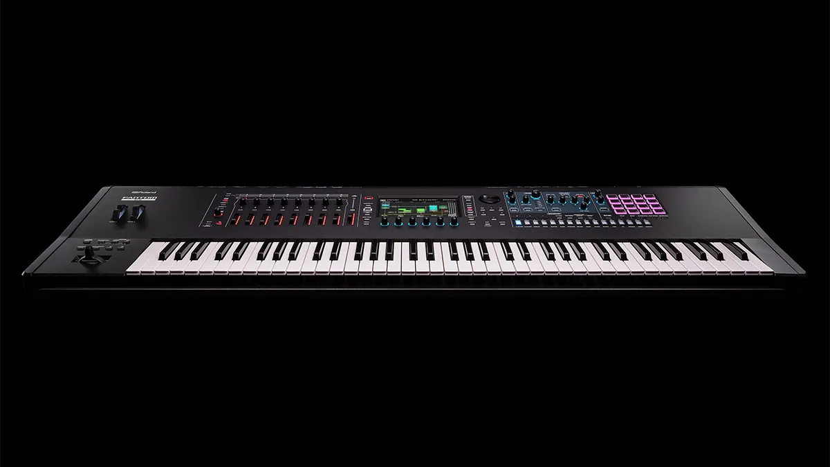
Now new users can get their EX kicks right out of the box
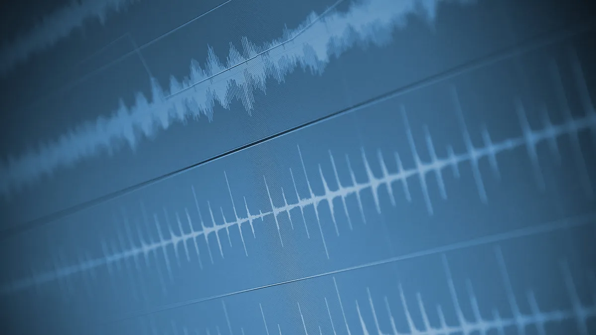
Company plans to develop advanced machine learning algorithms that can automatically detect musical instruments

Synth workstation? Karaoke machine? Recording studio in a ghetto blaster? Answer: all - and none - of the above…

For our latest free sample pack, we ran a variety of loops and one-shots through the Casio SK-1, Akai S900 and Bugbrand BugCrusher

“I guess we were sort of playing a game to see who could get the furthest behind without getting off beat,” says Saadiq of the recording of D’Angelo’s Lady

One of the world’s most popular studio microphones gets back to basics. We find out more

Do think twice, it’s the wrong mic

Is this your new best case scenario? We find out

“I brought this weird Roland monosynth upstairs. It was an early ’70s primitive synth and we were bugging out over it”

The late composer might have been known for his cutting-edge synth use, but he didn't agree with every studio breakthrough

Only one other producer has managed it

It seems that the streaming platform could be set to capitalise on the demand for multiple versions of viral hits
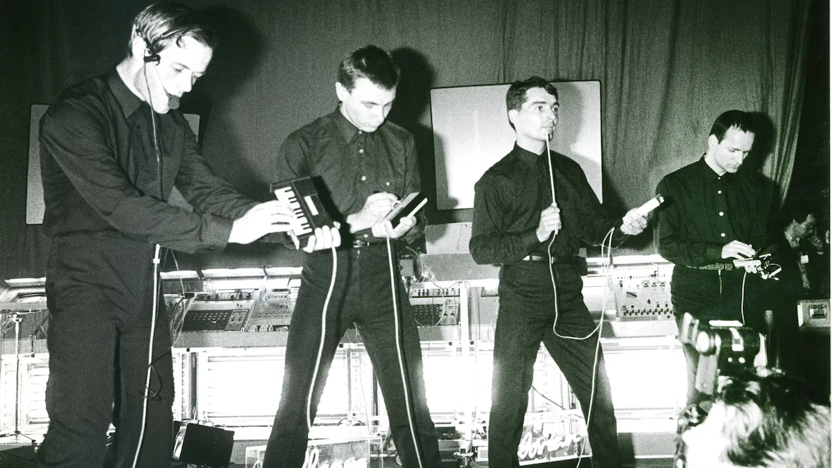
And it's certainly not the only piece of weird gear the iconic German band have used…

The DT-DX is based on the Raspberry Pi-powered MiniDexed DIY synth